Nearly a million fake black holes to understand two real ones

Imagine you want to train a program to recognize faces. It needs thousands of photos: lit by daylight, at night, in profile, blurred, wearing glasses. The program learns to ignore irrelevant variations and extract the features that matter. With black holes the problem is the same, except nobody knows exactly what they look like. And the face changes every few minutes.

The Event Horizon Telescope (EHT), the network of eight radio telescopes scattered across the planet that produced the first image of a black hole in 2019, collects enormously complex data. These are not photographs: they are interference measurements between pairs of telescopes, scattered pieces of information that need to be reconstructed. A research group led by Michael Janssen, in a paper published in Astronomy & Astrophysics, built a library of nearly a million simulated observations to train a neural network to interpret that data. The question driving the work is not “what does the black hole look like”, but something more subtle: how do you teach a program to recognize the physical properties of an object that never looks the same way twice?

The most realistic training ground ever built

Training a neural network requires labeled examples. In the case of the EHT, each example is a simulated observation of a black hole with known properties: how fast it spins, how magnetized its surrounding disk of matter is, the angle from which we are viewing it. The network learns to associate certain patterns in the data with certain values of these parameters, then applies them to real data.

The problem is that simulating an EHT observation does not mean taking a theoretical image and adding some noise. It means reproducing the entire signal path: atmospheric turbulence above each telescope, antenna pointing errors, water vapor in the skies over Chile and Hawaii, the loss of sensitivity when the atmosphere changes faster than the correction software can follow. Janssen and colleagues simulated all of this for two targets, the supermassive black holes Sagittarius A* (Sgr A*) at the center of the Milky Way and Messier 87 (M87*), producing 600,000 synthetic datasets for M87* and 252,000 for Sgr A*. In total, 962,000 fake observations with real labels.

The realism of the simulation is the key point. The synthetic data pass through the same calibration software used for real data, with the same flaws and the same corrections. If the calibration pipeline introduces an artifact in the real data, it introduces it in the synthetic data too. The network sees both and learns not to confuse them with physical signals.

When the enemy is the black hole itself

Telescope calibration has improved. The authors updated the EHT data reduction software, combining frequency bands and polarization channels more efficiently. The result is a 10 percent increase in measurement sensitivity across all telescope pairs, especially for the weakest signals. In practical terms, the new method manages to “see” connections between telescopes that were previously lost. A solid technical advance.

But the main obstacle to reading the physical properties of a black hole from the measurements is not instrumental noise, but how much black holes change over time.

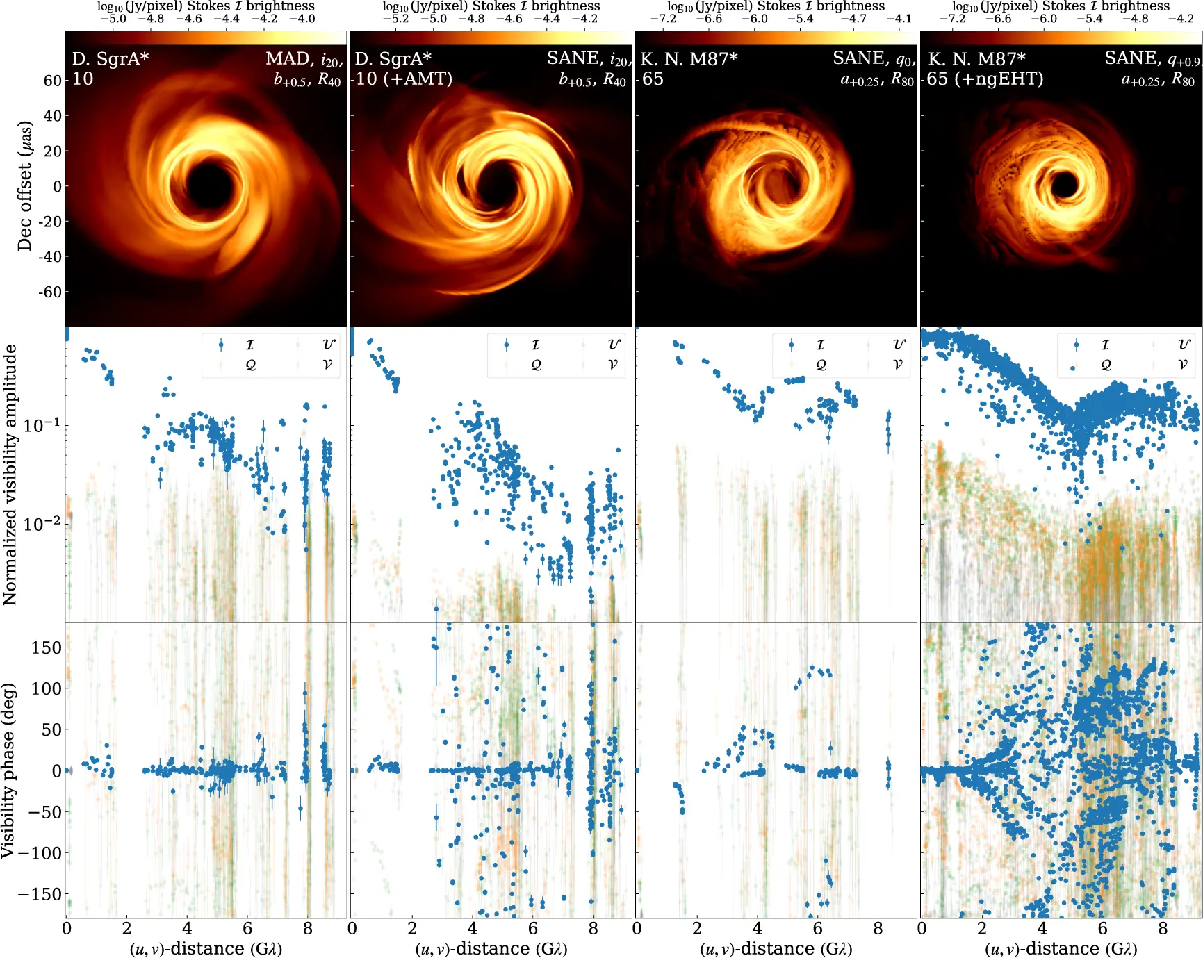
Sgr A* is an extreme case. The matter falling toward the black hole at the center of our galaxy changes configuration on timescales of minutes, because the black hole has a “small” mass by supermassive black hole standards, roughly four million times that of the Sun. The characteristic timescale of the fluctuations is about 20 seconds. A single EHT observation lasts 12 hours. In that time the black hole changes appearance hundreds of times. Simulating a single observation of Sgr A* requires 432 consecutive frames from the simulation.

M87* is more stable, with a characteristic timescale of eight hours, because it is 1,500 times more massive. A single frame is enough for an entire simulated observation. The stability is relative, though: on timescales of months and years, M87* changes too, and understanding how much it changes is one of the keys to distinguishing between models.

The photo that lies

The most instructive result in the paper concerns a specific model of Sgr A*: a black hole with intermediate spin, a strongly magnetized disk, viewed nearly face-on. This model, compared with the 2017 EHT data in a static way, passes all the selection criteria used by the EHT collaboration in previous analyses. It looks like a plausible candidate.

Then the authors look at variability over time. They generate three synthetic realizations of the same model over the span of an entire observing session, each starting from a different frame of the simulation, and compare them with the real measurements. The comparison uses closure phases: quantities derived by combining data from three telescopes in a way that cancels most instrumental errors. On some groups of three stations, the model matches the data well. On others, after midday, simulated and real data diverge sharply.

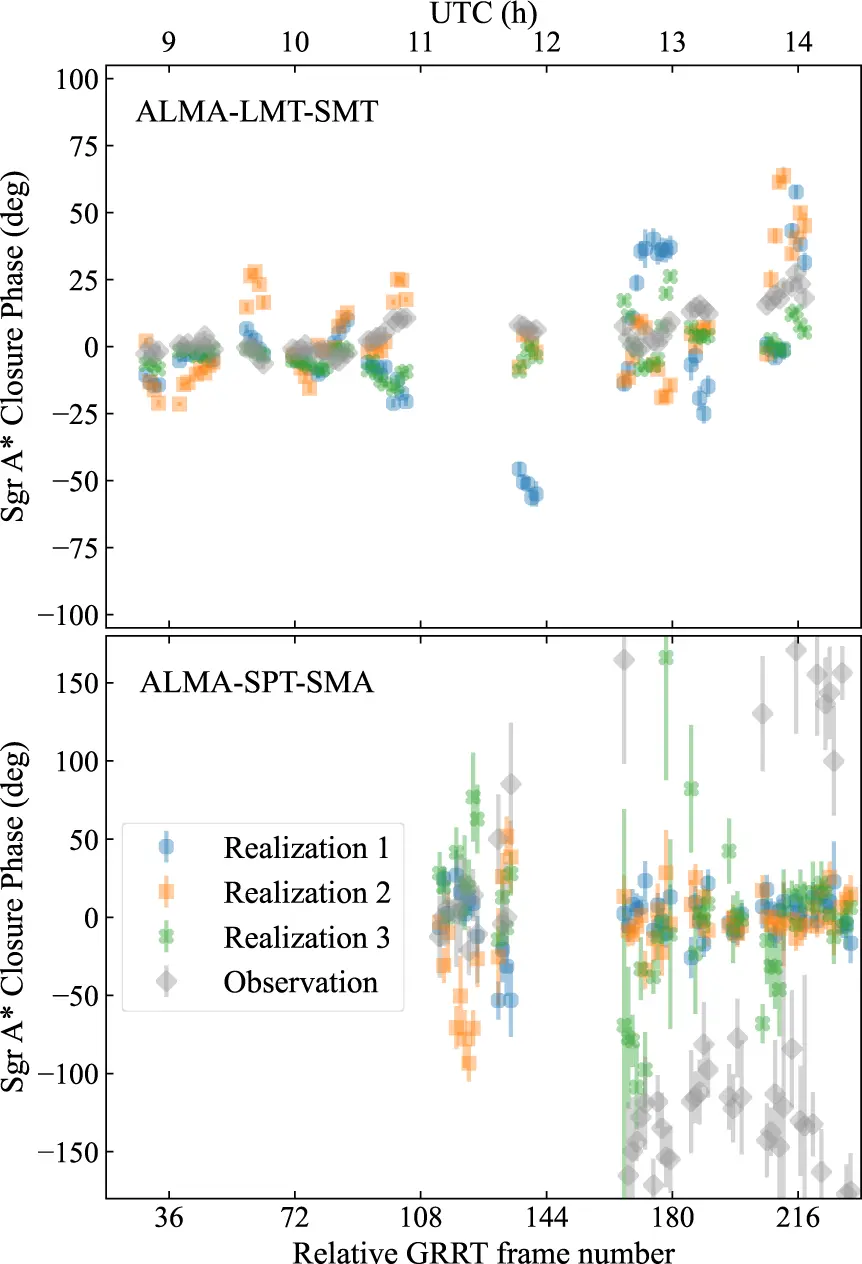
A photograph of the model looked right, but the film did not.

The models waiting for a better telescope

The simulated models cover a broad parameter space. The authors included standard black holes described by general relativity and two classes of “exotic” black holes: those with electric charge, and dilaton black holes, predicted by certain variants of string theory where gravity behaves differently near the horizon.

For the standard models, the behavior is predictable: strongly magnetized disks are more turbulent than weakly magnetized ones. Magnetic field eruptions produce violent brightness variations. Dilaton models are a separate case: they do not spin and never reach the strongly magnetized state, and a systematic comparison of their variability is deferred to future work.

For electrically charged black holes, the diagnostic signal is more direct. A sufficiently high charge reduces the size of the event horizon. The black hole’s shadow shrinks, and this reduction leaves an imprint in the interferometric signal: detecting it requires telescopes far enough apart from one another. With the network planned by the next-generation EHT (ngEHT) project, which will bring the total to 22 stations, the difference would become measurable.

What the network must learn to ignore

The direct comparison between synthetic data and the “perfect” theoretical model, reported in the paper’s appendix, reveals where residual instrumental noise hides. Total intensity signal amplitudes are reduced by variations in telescope sensitivity and imprecise pointing. Linear polarization is contaminated by signal that bleeds accidentally between polarization channels: the synthetic data show more polarization than the real signal, because the instrument creates artificial polarization. Circular polarization is almost entirely an instrumental artifact.

Closure phases, quantities that combine data from three telescopes in a way that cancels many instrumental errors, are stable instead. The difference between the synthetic data and the perfect model is minimal. This makes them the most reliable product for parameter inference, and probably the channel the neural network will rely on most.

Closure phases carry almost nothing but physical signal: amplitudes are already noisier, and circular polarization is almost entirely instrumental artifact. A neural network trained on realistic synthetic data can, in principle, learn this hierarchy on its own. If the synthetic data were not realistic, the network would learn a wrong hierarchy and then fail on real data.

Why one night is never enough

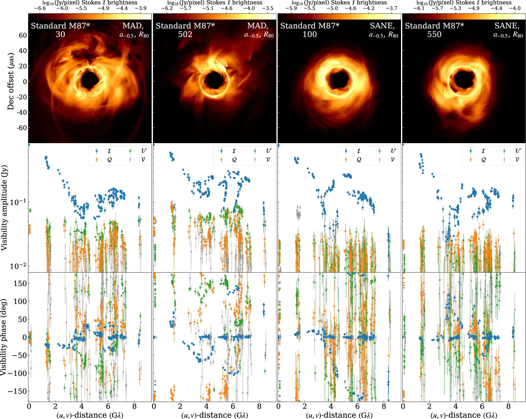
The paper devotes a section to distinguishing different M87* models through long-term monitoring. Three models with different parameters produce closure phases that, on a single observation, overlap. Over years of observations, the two strongly magnetized models separate from the weakly magnetized one by their degree of variability. The two strongly magnetized models distinguish themselves from each other by the median value of the closure phase, which depends on the black hole’s spin rate.

No single observation is enough: separating the models requires the movie, not the photograph. And a neural network trained on the full arc of model variability can, in principle, extract these differences even from single datasets, because it has seen enough examples to recognize the traces of variability even in an isolated “snapshot”. The authors anticipate that in the subsequent papers of the series, the neural network succeeds at this: a model trained on the first half of the observations correctly predicts the parameters of the second half.

The space between the data and the answer

This paper is the first of a series of three. It does not yet contain the actual inference, the one that will say “the black hole has this spin with this probability.” It contains the training ground, the rules of the game, and the first insights into what works and what does not.

The choice to build nearly a million synthetic datasets that faithfully reproduce the signal path, the instrumental errors, and the calibration is a heavy investment. Roughly 100 gigabytes of data for each source. The justification is simple: a neural network is as good as its training data, and for EHT data there are no shortcuts. The black hole changes face. The atmosphere changes. The telescopes make different mistakes every night. If the training ground does not capture all of this, the network learns a simplified world and then collides with reality.

One question remains that the paper does not address, because it belongs to the subsequent installments of the series: how robust is the result when the real black hole does not correspond to any of the models in the training ground? The parameter space is broad, but not infinite. General relativity predicts black holes described by mass, spin, and charge. If gravity works differently near the event horizon, the models in the training set might not contain the right answer. The network, in that case, would still give an answer.

---

References

Janssen, M. et al. (2025), Deep learning inference with the Event Horizon Telescope. I. Calibration improvements and a comprehensive synthetic data library, A&A, 698, A60. DOI: 10.1051/0004-6361/202553784