Near-zero errors, wrong answers

A program that analyzes data and tells you “I don’t know” is more useful than one that always gives an answer. This sounds obvious, but conventional neural networks do not do it by default. They produce a number: the black hole’s spin is 0.7. Period. No error bar, no indication of how confident the answer is. If the data is ambiguous, if two physically different models produce nearly identical signals, the network picks one anyway and does not warn you.

The team led by Janssen built a different kind of program, called Zingularity, published in Astronomy & Astrophysics. It is a Bayesian artificial neural network (BANN), a type of program where the internal weights, the numbers the network adjusts during training, are not fixed values but probability distributions. Each time the network analyzes a dataset, it produces not one answer but a spread of possible answers, each with its own probability. If the data is clear, the spread is narrow. If the data is ambiguous, the spread widens. And if the data looks nothing like anything the network has ever seen, the spread can split into two separate peaks, an explicit signal that says: I cannot choose.

The goal is to extract the physical properties of two supermassive black holes, objects so dense that not even light can escape their gravity, Sagittarius A* (Sgr A*) at the center of the Milky Way and Messier 87 (M87*), directly from data collected by the Event Horizon Telescope (EHT), the network of eight radio telescopes that produced the first image of a black hole in 2019. Not from the reconstructed images, but from the raw data: the interference measurements between pairs of telescopes, called visibilities, that carry the full polarization information of the light.

135 million parameters for five numbers

Zingularity’s architecture combines two ideas. The first half is a convolutional block (ResNet), a type of program designed to recognize patterns in structured data. The visibilities arrive sorted by telescope pair and time stamp, and the network learns which combinations of amplitudes and phases, measured on which telescope pairs, are most informative for each physical parameter. The second half is a series of fully connected variational layers, the ones that make the network Bayesian: each neuron does not have a fixed weight but a distribution, and at every pass the weight is drawn randomly from that distribution. The result is that, given the same observation, the network produces slightly different answers each time. A hundred passes give a hundred answers, and their distribution is the posterior: the network’s estimate together with its uncertainty.

For M87*, the network has 1 376 806 free parameters. For Sgr A*, which also requires estimating the disk inclination and position angle, it has 135 068 877. The numbers to extract are three or five: the black hole spin (how fast it rotates, which warps the surrounding space), the magnetic state of the matter disk (strongly or weakly magnetized), the ratio between ion and electron temperatures in the plasma. For Sgr A* the network also estimates the disk inclination and position angle. The disproportion is deliberate. A network with far more parameters than it needs to estimate has the freedom to find complex combinations in the data, patterns a smaller model would miss. Regularization, a mechanism that penalizes weights that grow too large or too numerous, prevents the network from memorizing the data instead of learning from it.

The training data comes from the synthetic library that Janssen and colleagues built in the first paper of the series: 600 000 datasets for M87* and 252 000 for Sgr A*, each a complete simulation of the signal path from source to telescope, including atmospheric effects, calibration errors, and cross-talk between polarization channels.

The perfect score that means nothing

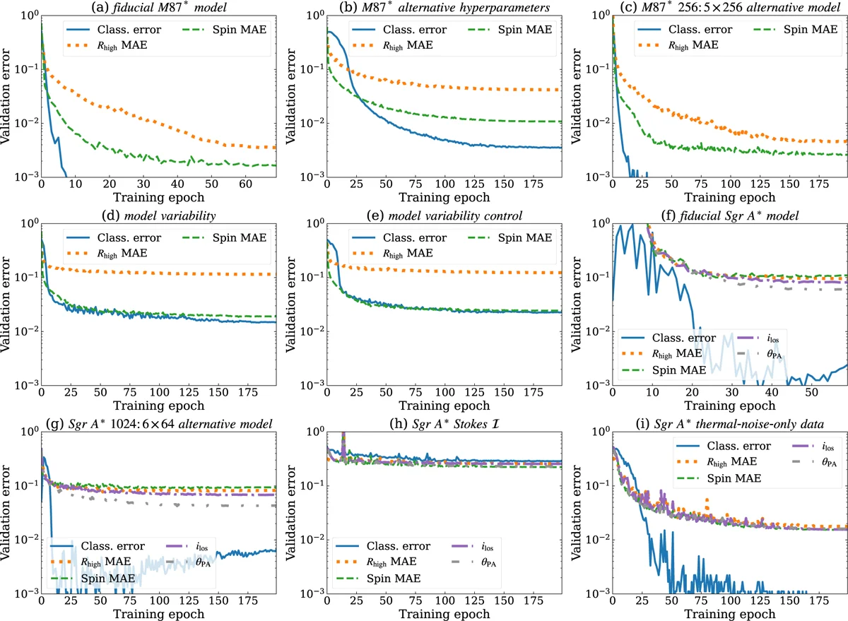
Here is the paradox. When the authors train a version of the network using only thermal noise, the simplest form of disturbance in the data, without the other signal corruption effects, the validation errors drop. The network distinguishes nearly perfectly between models with strong and weak magnetic fields, estimates the spin with minimal error, classifies everything with precision.

The result is useless.

A network trained on data that is too clean learns to exploit features of the signal that in real data are masked or distorted by effects the simplified synthetic data never contained. Atmospheric turbulence, variations in telescope sensitivity, cross-talk between polarization channels: everything the network has never seen becomes a source of invisible systematic error. The program is confident in its answers, because the uncertainties are calibrated to a world simpler than the real one. The error bar is narrow. Around the wrong answer.

The authors show this by comparing training curves. With the full data, the M87* network takes 70 epochs and the Sgr A* network 50 or 60 (one epoch is one complete pass through the training set), and the validation errors settle at finite, measurable values. With the simplified data, the errors drop faster and lower. The difference is not a defect in the network: it is a defect in the data. When the training set does not contain the full complexity of the real world, the program has no way of knowing it is learning an incomplete version of reality.

When polarization makes the difference

Polarization, the direction in which the electromagnetic wave oscillates, is the information channel that sets Zingularity apart from previous attempts. Neural network analyses of EHT data published so far used only the total intensity of the light (Stokes I parameters). Janssen and colleagues included all four Stokes parameters: total intensity, linear polarization in two directions, and circular polarization. Eight input channels in total, real and imaginary parts of each correlation product.

The difference is sharpest for classifying the magnetic state of the disk. Without polarization, Sgr A* models with strong and weak magnetic fields produce intensity signals that look alike. The network trained on total intensity alone struggles to tell them apart, and the classification errors remain high. With full polarization, the classification becomes nearly perfect. A strong magnetic field leaves an imprint in linear and circular polarization that is absent in weak-field models: the network learns to recognize it.

For estimating the black hole spin, the effect of polarization is less pronounced but still present. The ion-to-electron temperature ratio in the plasma, the hardest parameter to estimate for M87* models, has the highest validation errors regardless of the data used. The effect of this parameter on the images is subtle: for M87*‘s strongly magnetized models, the ion-to-electron temperature ratio barely changes the image morphology, and the little it does change is hard to catch with the 2017 EHT coverage.

Two codes, same equations, different answers

The most severe validation does not come from within the dataset, but from outside it. The authors generated test data with a simulation code different from the one used for training. The training data comes from KHARMA; the test data comes from BHAC-RAPTOR. Both solve the equations of general relativistic magnetohydrodynamics, the equations describing how magnetized plasma moves near a black hole, but with different numerical implementations: different ways of slicing the computational grid, different approximations for radiative transfer (how light travels through matter on its way from the source to the telescope), different choices for the electron temperature.

For M87*, the test is passed. The network trained on KHARMA correctly identifies the magnetic state and estimates the spin of the BHAC-RAPTOR models with small errors. The posterior is narrow and centered on the right value. The two simulations, despite being independent, produce signals similar enough on the scales the network uses to decide.

For Sgr A*, the result is more interesting. A model with a strong, organized magnetic field (MAD), mildly negative spin, and intermediate inclination gets identified by the network as a model with a weaker, more turbulent magnetic field (SANE), strongly negative spin, and different inclination. The true parameters fall between grid points of the training data: no model in the training set has exactly those values. The network, faced with a signal it has never seen, matches it to the closest model it knows. The problem is that “closest in the interferometric data” does not mean “closest in physics”. Two black holes with opposite magnetic properties can produce nearly identical visibilities through the EHT’s eight telescopes, because eight telescopes produce too few measurement pairs to catch the differences.

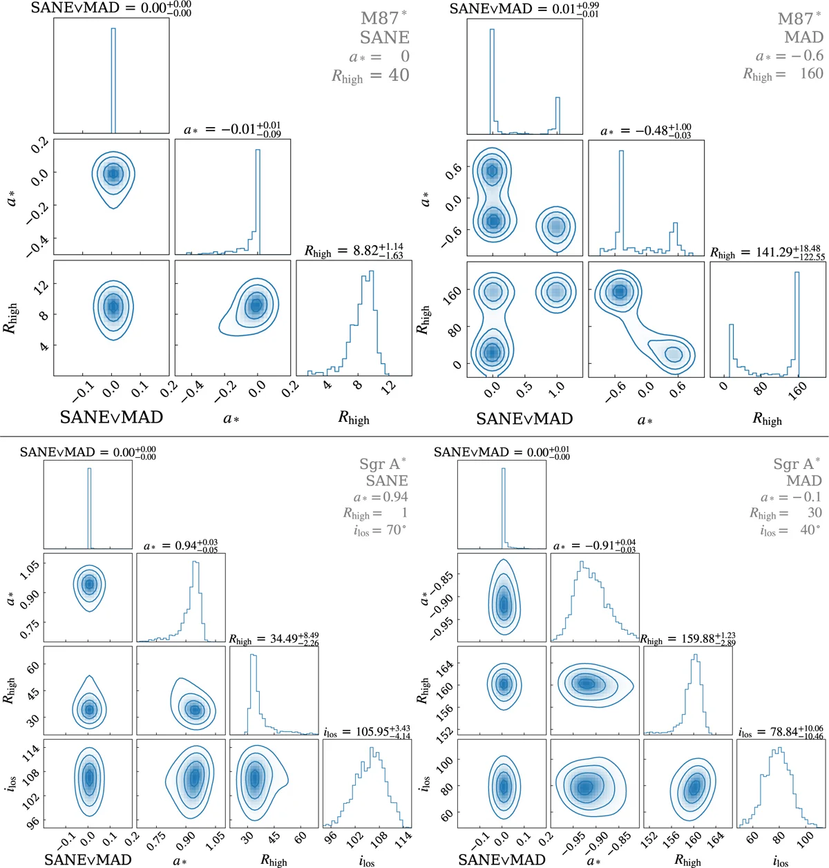
The Bayesian nature of the network works halfway here. The posterior for the correctly identified model is narrow and centered. The posterior for the misidentified model is also narrow, but centered on the wrong value. The network does not “know” that it does not know, because the signal does resemble a model in the training set. The honest failure mode, where the posterior splits into two peaks signaling ambiguity, appears only when the test data is an M87* model with parameters at the edge of the grid: the network sees two equally plausible models and declares it. For Sgr A*, the confusion is more insidious, because the interferometric signals of the two models are too similar to distinguish.

The comparison between simulations from different codes tests how much the method depends on the choice of simulation, not its ability to generalize to real EHT data. Real data contains additional effects, including the intrinsic variability of Sgr A* on the gravitational timescale of about 20 seconds, that none of the simulations fully reproduce.

The slowest program that beats everything

An underappreciated aspect of Zingularity is speed. Training is the expensive piece, but once trained, inference is nearly instantaneous. Obtaining 100 posteriors from 100 bootstrap resamplings of the EHT data takes 20 seconds on a single GPU. The comparison with the traditional methods used by the EHT collaboration is stark: those require comparing the observed data against hundreds of thousands of models one at a time, averaging over a subset of instrumental effects to isolate the physical signal. It is a process that demands far more computational resources and that, for cost reasons, often explores only part of the parameter space.

Zingularity explores the full parameter space of the magnetohydrodynamic and radiative transfer models in a single pass. And it does so while accounting, in the training data, for the entire signal path. The traditional alternative, to achieve the same result, would require marginalizing over all instrumental effects for every model, a computation that with current data would be prohibitive.

The speed comes at a cost. The network is tied to the models it was trained on. If the real black hole has properties not covered by the simulation grid (a different chemical composition, magnetic reconnection (the sudden breaking and reassembly of magnetic field lines, which releases energy), a disk tilted relative to the rotation axis), the network has no way of knowing. It gives the closest answer it knows, with an uncertainty calibrated to a universe of possibilities that may not contain the right one.

The gap between the score and reality

The paper closes by stating that it is easy to achieve low validation errors on synthetic data with neural networks, particularly when the forward modeling is too simplified. The sentence applies well beyond the EHT. Every application of machine learning to real scientific data runs into the same problem: the synthetic training data is a model of reality, and every model has limits. The difference between a good program and a dangerous one is the ability to signal when those limits have been reached.

Zingularity does this in two ways: through Bayesian posteriors, which widen or split when the data is ambiguous, and through bootstrapping, a resampling of the observed data that propagates instrumental uncertainties all the way to the final answer. Neither mechanism is perfect. The narrow posterior around the wrong answer, as in the misidentified Sgr A* model, shows the network can fail silently when the data resembles something different too closely. The application of these networks to the actual EHT data, with the results on the physical properties of the two black holes, is the subject of the third paper in the series, published alongside this one in Astronomy & Astrophysics.

The 135 million parameters of the Sgr A* network converge on five numbers. The open question is whether those five numbers describe the black hole that is there, or the most similar black hole among those the network learned to recognize.

---

References

Janssen, M. et al. (2025), Deep learning inference with the Event Horizon Telescope. II. The ZINGULARITY framework for Bayesian artificial neural networks, A&A, 698, A61. DOI: 10.1051/0004-6361/202553785

Code: Zingularity on GitLab